EECE 5550 Mobile Robotics

Lecture 5

Uncertainty & Kalman Filter

Dr. Xian Li

Department of Electrical and Computer Engineering

Northeastern University

Example: measure weight with imperfect scales

An example to understand fusing two noisy measurements

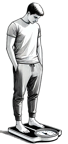
A person standing on a bathroom scale

Fact: Scale A is good to ±2 lb, scale B to ±5 lb, and neither is biased.

Measurement: Scale A reads "160 lbs", while Scale B reads "170 lbs".

What can we conclude about your weight?

Well, what are our choices?

  • Choose a number less than both A and B.
  • Choose a number greater than both A and B.
  • Choose to only trust A, and assign 160lbs to our weight estimate.
  • Choose to only trust B, and assign 170lbs to our weight.
  • Choose an average number: 165 lb ± 2.7 lb
  • Weight each by how much you trust it: 161.4 lb ± 1.9 lb

➔ If neither scale is biased, each one's error is as likely to be high as low.

➔ Nothing points you outside the two readings.

➔ Ignoring a measurement throws away information, and it only makes sense if that scale is useless.

➔ Probably wrong, but reasonable

➔ A better estimation: weighted average!

2

Try it: fuse two scales

Move the readings and uncertainties. The weighted average trusts each scale by 1/σ².

Scale A

Scale B

x^= zA/σA2+zB/σB2 1/σA2+1/σB2
3

EECE 5550 Mobile Robotics

Where is the robot?

The robot faces a wall. Two estimates of the distance disagree.

2.00 m

odometry

Integrated from the wheels since a known start. Its error has been growing the whole way: σ ≈ 5 cm.

2.03 m

LiDAR

One beam, straight at the wall, right now. Your Lab 2 sheet says about 1% of range: σ ≈ 2 cm.

?

your answer

Pick one, average them, or something better. You will learn an “optimal” way: Kalman Filter

By the end of today you can answer this with a number and an error bar, and say why the error bar is smaller than either one.

4

EECE 5550 Mobile Robotics

2

Today

How to combine two estimates that are both wrong, and end up less wrong than either?

❏Belief is a distribution

❏Propagating uncertainty

❏Bayes’ rule, working form

❏The recursive Bayes filter

❏The Kalman filter

Reading

[1] How a Kalman filter works, in pictures

[2] Kalman FIlter Tutorial

[3] Probabilistic Robotics, by Dieter Fox, Sebastian Thrun, and Wolfram Burgard

[4] GitHub Repo: Kalman-and-Bayesian-Filters-in-Python

Problem Set 2 and Lab 2 & 3

SECTION 1

Belief is a distribution

Mean, variance, covariance, the ellipse

A simple example

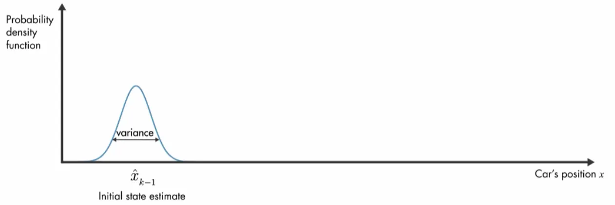
Belief: A probability distribution that models uncertainty over possible states X of the world

Suppose I roll a fair die, but don’t tell you the result X

Q1:  What should your belief be about X?

A1: Prior: p(X=x)=⅙ for all x in {1, …, 6}

Q2:  Suppose that now I look at X, and tell you that its value is even.  What should your belief be now?

A2: Posterior (conditional): p(X=x|X in {2,4,6}) = p(X=x)p({2,4,6})=1/3

Key point: In this example, it is not the world that is changing, but rather our information about the world!

Remember: Beliefs model our state of knowledge of the world

p(X) X A blue dice cup tipped over next to two dice
7

Try it: update a belief

I roll a hidden die. Ask questions and watch your belief change. The die never changes; only what you know about it does.

Ask about the roll

    8

    EECE 5550 Mobile Robotics

    5

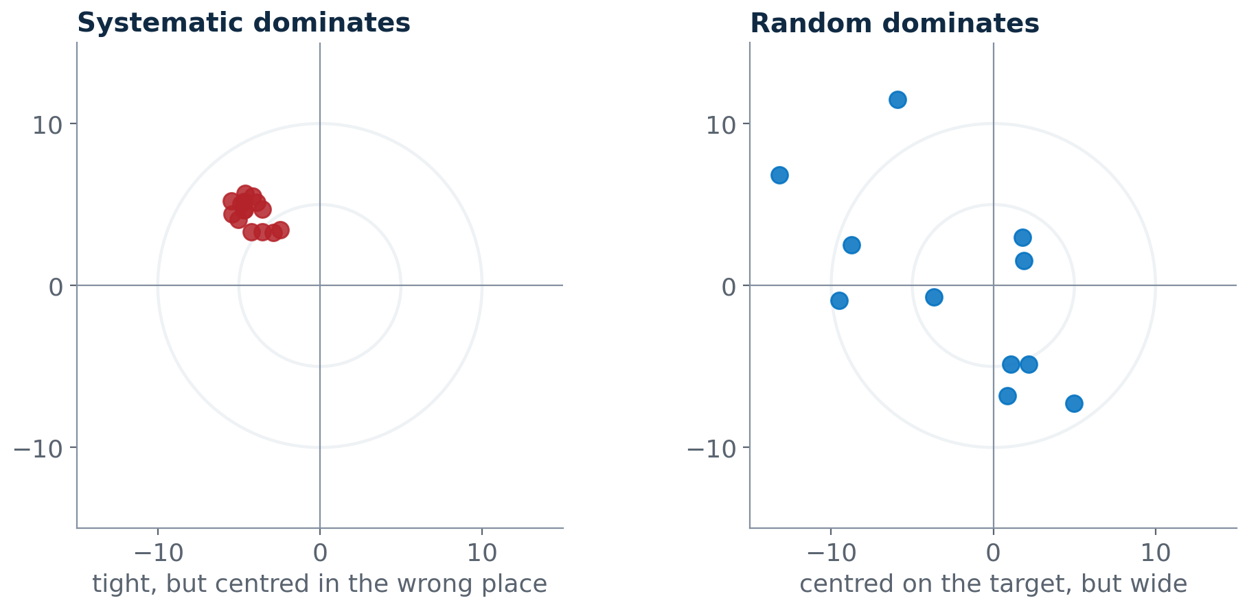
    Systematic error V.S. Random error

    Lecture 4 removed the shift. Today is about the spread

    Systematic error: the shift

    Same every run. UMBmark measures it and calibration removes it. Lecture 4 and Lab 2 Task 3.

    Random error: the spread

    Different every run, so no calibration can remove it. The best you can do is know how big it is, carry that through every calculation, and combine sources to shrink it.

    Question: Difference between Accuracy & Precision?

    EECE 5550 Mobile Robotics

    5

    Systematic error V.S. Random error

    Lecture 4 removed the shift. Today is about the spread

    Systematic error: the shift

    Same every run. UMBmark measures it and calibration removes it. Lecture 4 and Lab 2 Task 3.

    Random error: the spread

    Different every run, so no calibration can remove it. The best you can do is know how big it is, carry that through every calculation, and combine sources to shrink it.

    Low accuracylow precision−10−10001010wide, and off the targetLow accuracyhigh precision−10010tight, but off the targetHigh accuracyhigh precision−10010tight, and on the targettrue valueestimates

    Question:

    What does “high accuracy, low precision” look like?

    EECE 5550 Mobile Robotics

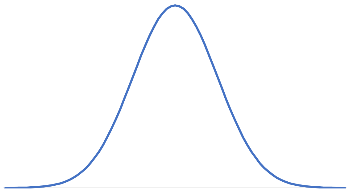
    The robot's belief is a distribution, not a number

    p(x)=1σ2πexp(−(x−μ)22σ2)

    Mean μ: the best single guess

    Variance σ²: how unsure; σ is in the same units as x

    Gaussian (Normal) Distribution

    EECE 5550 Mobile Robotics

    The robot's belief is a distribution, not a number

    Every estimate on a robot should come with its σ. A position without an error bar cannot be combined with anything.

    p(x)=1σ2πexp(−(x−μ)22σ2)

    Mean μ: the best single guess

    Variance σ²: how unsure; σ is in the same units as x

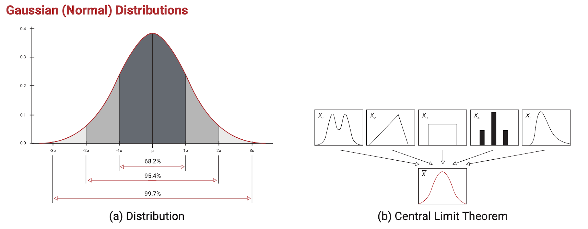
    Within 1σ, 2σ, 3σ: 68.27%, 95.45%, 99.73% of the time

    Gaussian (Normal) Distribution

    EECE 5550 Mobile Robotics

    5

    Why Gaussian?

    Assume Gaussian because it is usually close and always convenient. Then check whether your data agree.

    EECE 5550 Mobile Robotics

    5

    Why Gaussian?

    Assume Gaussian because it is usually close and always convenient. Then check whether your data agree.

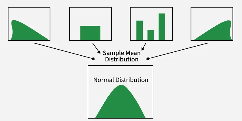
    Central limit theorem

    Odometry adds thousands of small, independent wheel errors. Their sum tends to a Gaussian whatever each one looks like

    EECE 5550 Mobile Robotics

    5

    Why Gaussian?

    Assume Gaussian because it is usually close and always convenient. Then check whether your data agree.

    The math closes

    A linear map of a Gaussian is Gaussian. A product of two Gaussians is Gaussian. So a filter that starts Gaussian stays Gaussian, and two numbers, μ and σ, describe it completely.

    EECE 5550 Mobile Robotics

    5

    Why Gaussian?

    Assume Gaussian because it is usually close and always convenient. Then check whether your data agree.

    When it fails

    A slip is one big error, not many small ones.

    Kidnapped Robot Problem.

    EECE 5550 Mobile Robotics

    Demo: beam_watch.py

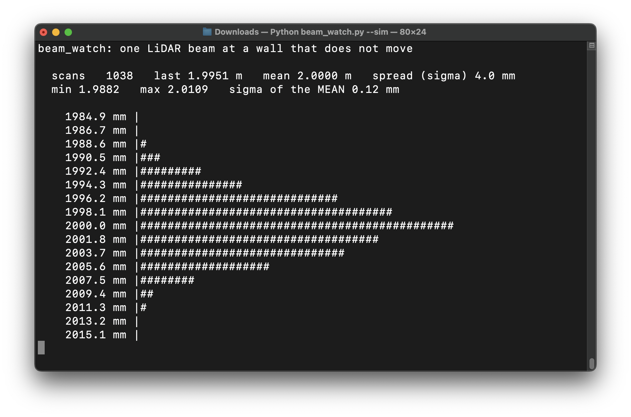
    The robot sits 2 m from a flat wall. Nothing moves. Watch the one beam that points at it.

    The wall does not move; the number does

    Your beam_watch.py, simulated: one LiDAR beam at a wall 2.00 m away, noise 4 mm.

    Python starts when the lecture gets close to this slide.

    Run

    Your script uses 4 mm. Changing it restarts the run.

    Python not started yet.
    18

    Gaussians

    Univariate
    p(x)∼N(μ,σ2):
    p(x)=12πσe−12(x−μ)2σ2
    μ − σμμ + σ68%x
    Multivariate
    p(𝐱)∼N(𝛍,𝚺):
    p(𝐱)=1(2π)d/2|𝚺|1/2e−12(𝐱−𝛍)T𝚺−1(𝐱−𝛍)
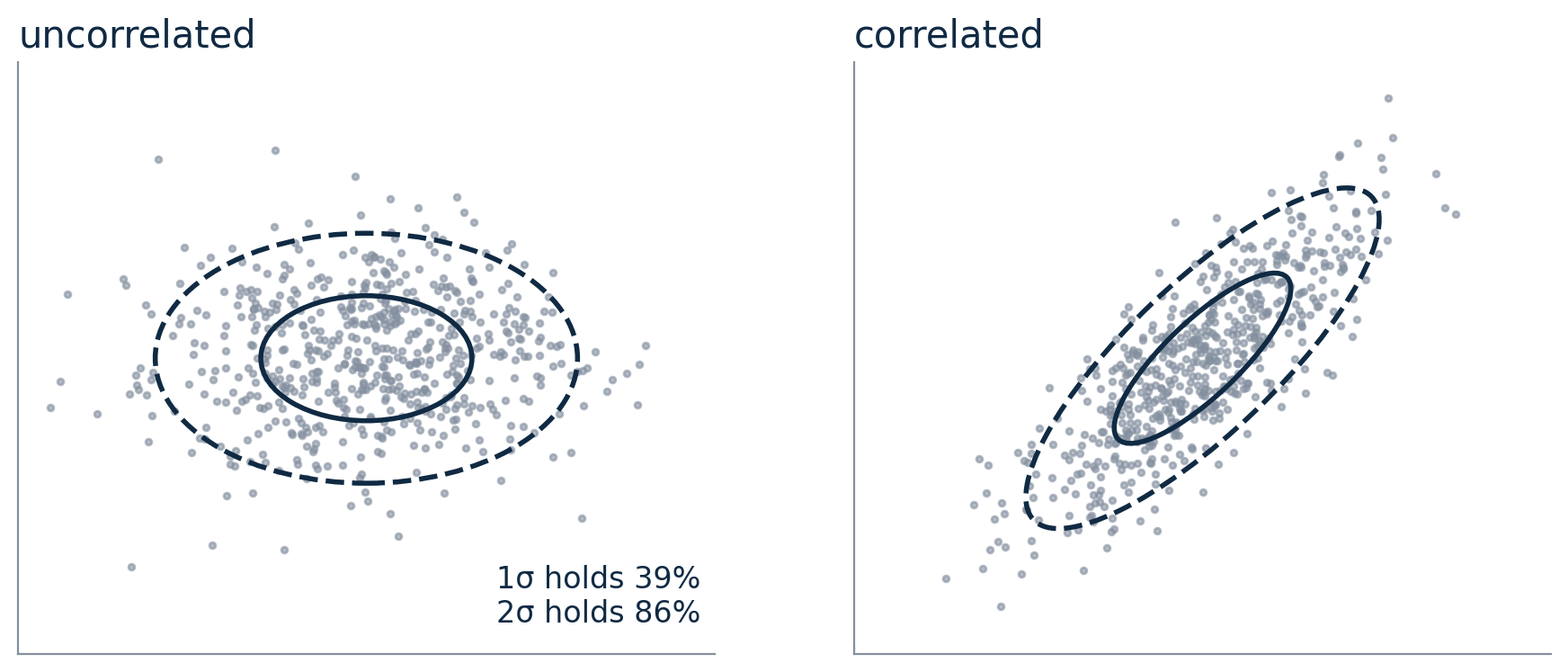
    x₁x₂𝛍1σ, 2σ, 3σ contours
    19

    EECE 5550 Mobile Robotics

    5

    Gaussians

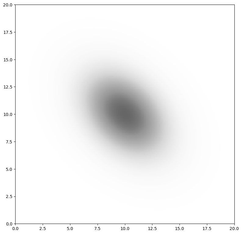
    2D case

    Σ=[σx2σxyσxyσy2],ρ=σxyσxσy

    Diagonal: the variance of each coordinate on its own

    Off-diagonal σxy: whether an error in x comes with an error in y

    ρ between −1 and 1: 0 means independent; ±1 means one determines the other

    In 2D, the 2σ ellipse holds 86% of the samples, not 95%. The 1σ ellipse holds only 39%.

    Gaussians

    2D case

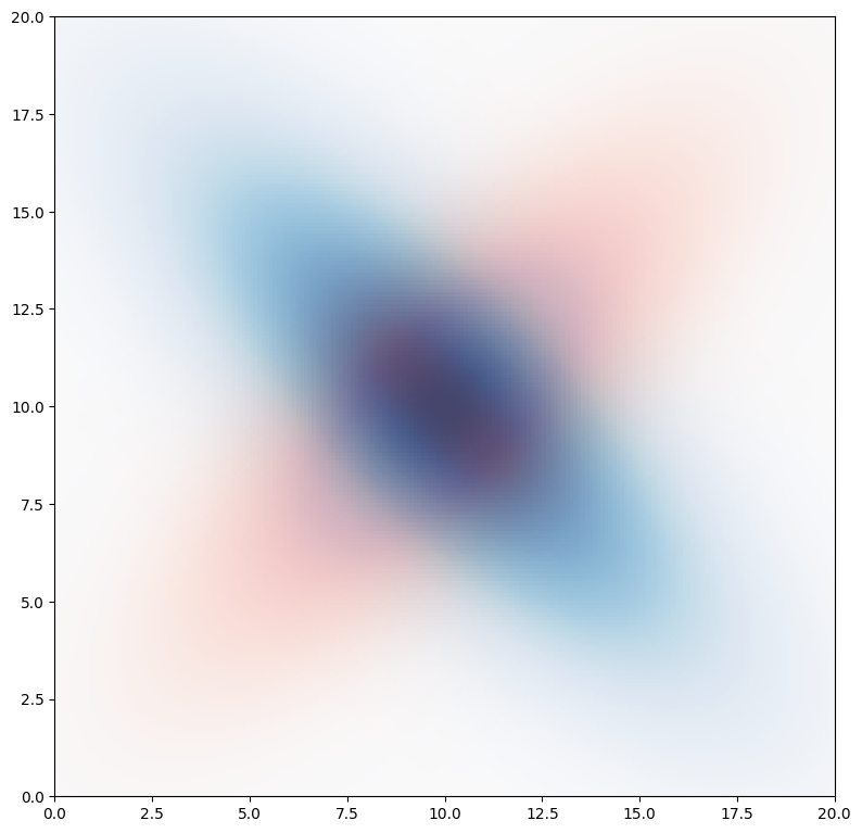
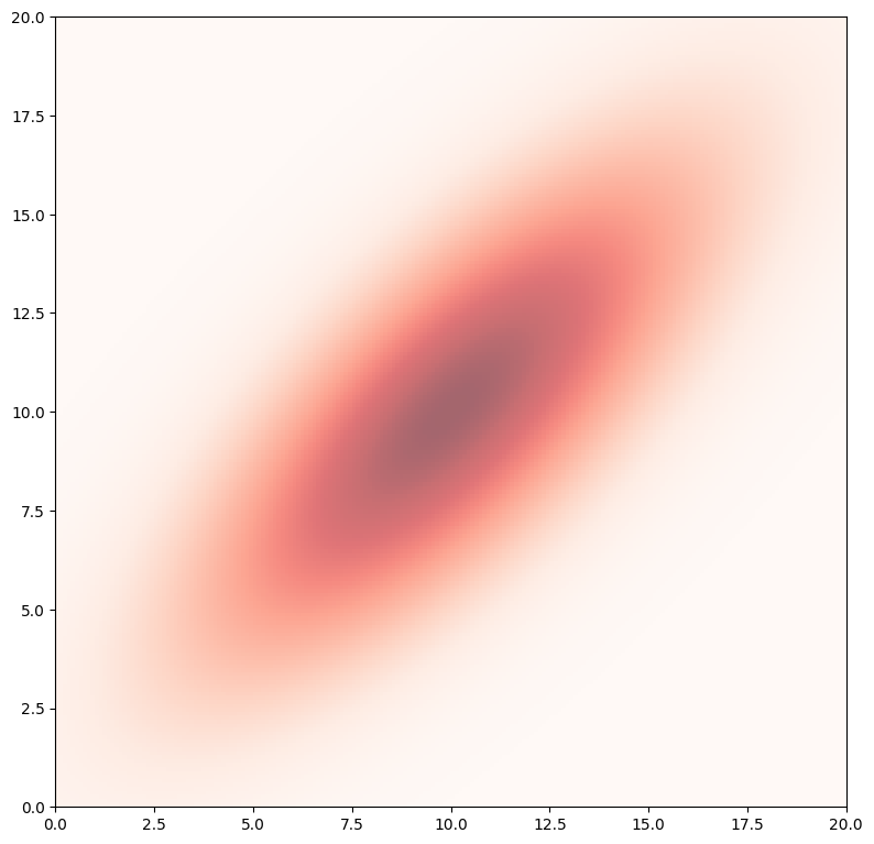
    Σ=[σx2σxyσxyσy2],ρ=σxyσxσy

    shading: the joint density p(x, y); top and right: the marginals p(x) and p(y)
    21

    SECTION 2

    Propagating uncertainty

    Model. Why odometry error grows sideways, and the banana

    EECE 5550 Mobile Robotics

    5

    Uncertainty

    Two rules carry it through any calculation

    Errors scale

    Convert a wheel's ticks to meters with a = 2πr / 508.8, and the tick noise is scaled by the same a. A 1% error in r is a 1% error in every distance.

    Variances add

    Two independent errors add in variance, not in size. Five steps of 1 cm each give √5 = 2.2 cm, not 5 cm. That is why random error grows as √n.

    Odometry is a long sum of small steps. Its random error grows like a square root, and its systematic error grows in a straight line.

    y=ax+b⇒σy=|a|σxz=x1+x2⇒σz2=σ12+σ22

    EECE 5550 Mobile Robotics

    5

    Uncertainty

    The same rule, for vectors

    𝐲=A𝐱⇒Σy=AΣxAT

    A maps the old variables to the new ones

    A Σ A-transpose is the only formula you need: it covers scaling, adding, and the cross terms

    Check: with A = [a] it gives σ² = a²σx²; with A = [1 1] and independent inputs it gives σ1² + σ2²

    EECE 5550 Mobile Robotics

    5

    Motion model

    Your TurtleBot uses this one

    x′=x+dcos(θ+Δθ2)y′=y+dsin(θ+Δθ2)θ′=θ+Δθd=dr+dl2,Δθ=dr−dlw

    Inputs u: the two wheel distances

    dr and dl, from /wheel_ticks. Each carries its own small random error.

    State x: the pose

    x, y, θ. The cos and sin of θ are what make the model nonlinear.

    +xr

    +yr

    θ

    (x,y)

    O

    +y

    EECE 5550 Mobile Robotics

    5

    Motion model

    Linearize: the Jacobian of one step

    x′=x+dcos(θ+Δθ2)y′=y+dsin(θ+Δθ2)θ′=θ+Δθd=dr+dl2,Δθ=dr−dlw

    +xr

    +yr

    θ

    (x,y)

    O

    +y

    Fx=∂f∂(x,y,θ)=[10−dsinϕ01dcosϕ001],ϕ=θ+Δθ2

    Derivative

    A heading error moves the end of the step in x & in y

    An error you already have is carried forward unchanged.

    If you were 2 cm off before the step, you are still 2 cm off after it.

    A position error cannot change the heading.

    Question: Why ?

    (θ+Δθ2)

    EECE 5550 Mobile Robotics

    Motion model

    One step of covariance propagation

    P′=FxPFxT+FuQFuT,Q=[k|dr|00k|dl|]

    First term: old uncertainty, carried forward

    Each robot drives d along its own heading, so a heading error becomes a sideways error. Nothing new is added: the ellipse is sheared, not enlarged.

    Second term: new uncertainty, added

    Each wheel rolls a little more or less than measured; that is Q. F_u turns those wheel errors into pose errors, mostly heading. This is the only term that makes the robot less certain.

    Motion model

    One step of covariance propagation, drawn two ways. Errors are exaggerated so the effect is visible.

    1. Before the step

    before: y and θ unrelated

    2. First term: carried forward

    first term: a shear

    3. Second term: new wheel noise

    second term: it grows

    dots: 700 simulated robots; color: each one’s heading error, right (blue) to left (amber); ellipses: 2σ. Click to switch between the robots’ positions and the y, θ plane.
    28

    EECE 5550 Mobile Robotics

    Drive straight, and the ellipse grows sideways

    ​

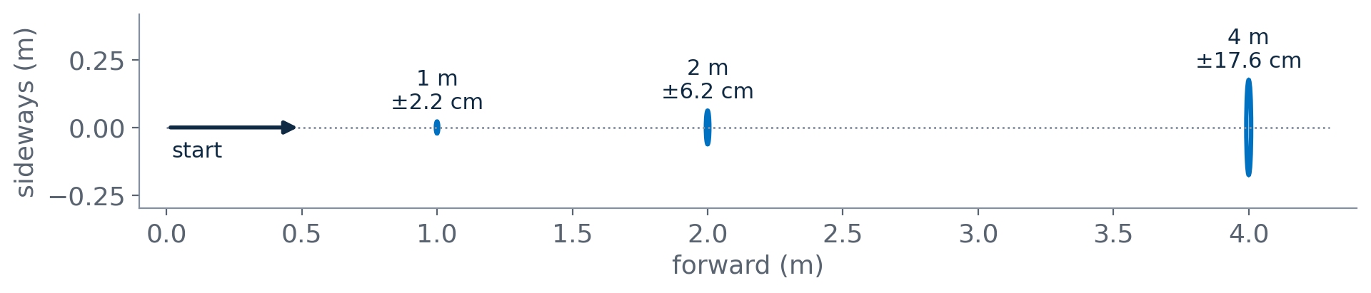
    1 m

    2 m

    4 m

    doubling

    along the path, σx

    0.22 cm

    0.32 cm

    0.45 cm

    ×1.414

    sideways, σy

    1.1 cm

    3.11 cm

    8.79 cm

    ×2.828

    heading, σθ

    1.09°

    1.54°

    2.18°

    ×1.414

    The pattern

    σx grows like √s, but σy like s√s.

    ​

    Problem Set 2 Problem 2 derives both.

    Odometry's uncertainty, propagated live

    Your cov_odom.py on a simulated TurtleBot: every step adds wheel noise to P, and the 2σ ellipse grows.

    Python starts when the lecture gets close to this slide.

    Drive

    Uncertainty

    Python not started yet.
    30

    EECE 5550 Mobile Robotics

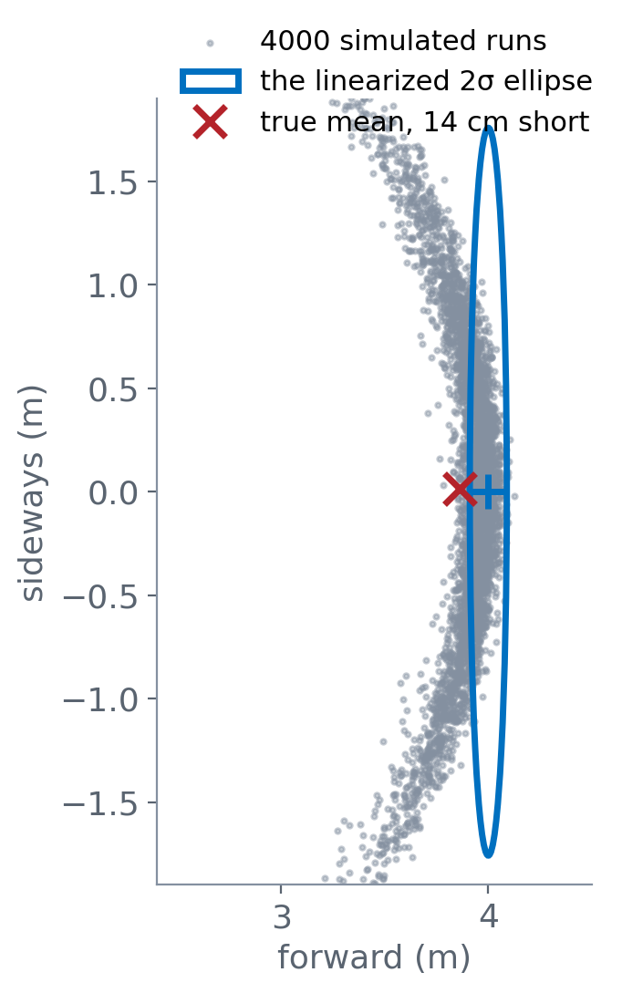
    The true shape is a banana

    Run the noisy motion 4000 times

    Heading errors bend each run into an arc, so the cloud curves back toward the start.

    ​

    ➔Linearizing gives an ellipse.

    ➔Without linearizing, the true spread is a banana whose two ends curl back toward the start,

    ​

    (Noise exaggerated here so the shape shows: σθ = 21.7°.)

    Question: Why bending backwards?

    ➔Taylor Series

    ➔Linearizing keeps only the first-order terms.

    ➔The first term the linearization drops is −dθ²/2, in x.

    ➔It's never positive. θ² ≥ 0

    ➔So, backwards

    SECTION 3

    Bayes' rule, working form

    Measurement. Two Gaussians become one

    EECE 5550 Mobile Robotics

    5

    Bayes' rule: how a measurement changes a belief

    p(x∣z)⏟posterior=p(z∣x)⏞likelihoodp(x)⏞priorp(z)

    prior

    What you believed before looking.

    ​

    Here: odometry.

    likelihood

    How probable this reading is, for each possible true distance.

    ​

    Here: the LiDAR model.

    posterior

    What you believe after. Prior times likelihood, rescaled to integrate to 1.

    p(z) does not depend on x. It only rescales, so in practice: posterior ∝ likelihood × prior.

    Rev. Thomas Bayes

    EECE 5550 Mobile Robotics

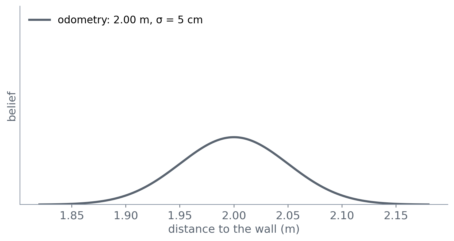
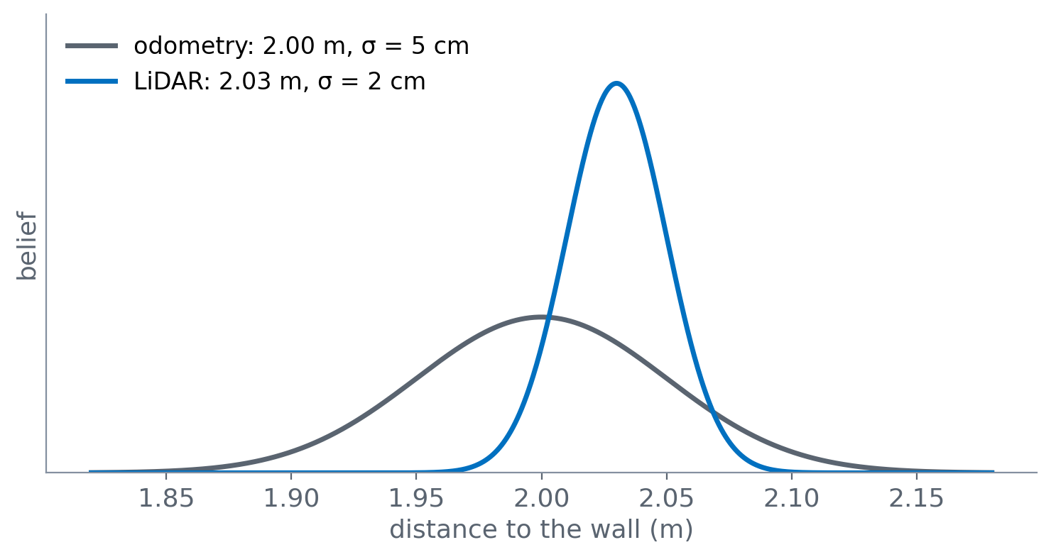
    The prior: what odometry says

    Odometry: 2.00 m, σ = 5 cm. Wide, because it has been accumulating error since the start.

    34

    EECE 5550 Mobile Robotics

    The likelihood: what the LiDAR says

    LiDAR: 2.03 m, σ = 2 cm. Narrow, because it measures the wall directly, right now.

    35

    EECE 5550 Mobile Robotics

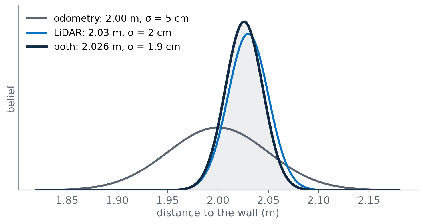
    The posterior: both, multiplied

    Both: 2.026 m, σ = 1.9 cm. Closer to the LiDAR, because it is more certain, and narrower than either.

    36

    EECE 5550 Mobile Robotics

    Two Gaussians multiply into one: the precision-weighted mean

    μ=σl2μo+σo2μlσo2+σl2=μo+σo2σo2+σl2⏟K(μl−μo),1σ2=1σo2+1σl2

    ​

    value

    where it comes from

    weight on the LiDAR, K

    0.862

    25 / (25 + 4), in cm²

    posterior mean

    2.026 m

    2.00 + 0.862 × 0.03

    posterior σ

    1.9 cm

    1/σ² = 1/25 + 1/4, in cm⁻²

    The weights are not 50/50.

    Each estimate is weighted by its precision, 1/σ², so a sensor twice as certain counts four times as much.

    37

    SECTION 4

    The recursive Bayes filter

    Predict, update, repeat

    EECE 5550 Mobile Robotics

    5

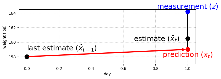
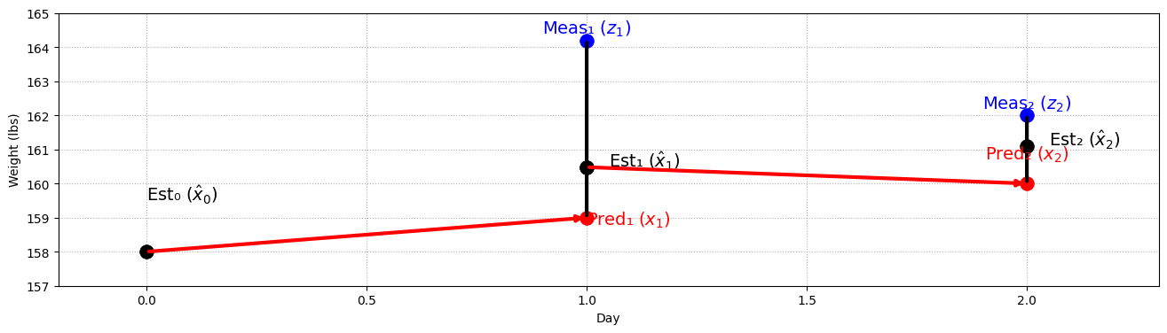
    Example: measure weight with imperfect scales

    What if we only have one imperfect scale?

    ​

    ​

    Go on

    Multiple measurements!

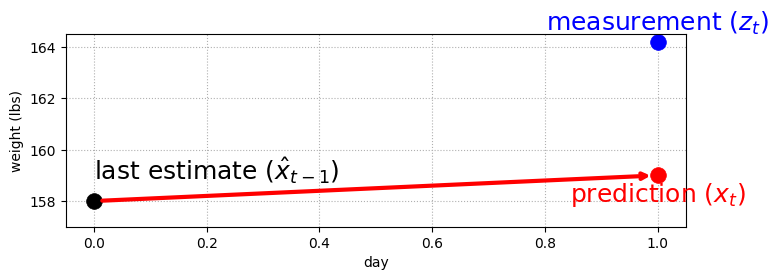
    Easimate based on prediction and measurement.

    Example: measure weight with imperfect scales

    A person standing on a bathroom scale
    Day 0Day 1Day 2Day 3Day 4Day 5Day 6Day 7Day 8Day 9Day 10
    Initialization!
    Question: What are Day 2’s Estimate & Prediction for Day 3?
    Question: What are Day 4’s Estimate & Prediction for Day 5?
    DayMeasurementPredictionEstimateTruth
    0
    -
    -
    -160.0
    160.0
    1
    158.0
    161.0
    159.8
    161.0
    2
    164.2
    160.8
    ?1162.16
    162.0
    3
    160.3
    ?2163.16
    162.02
    163.0
    4
    159.9
    163.02
    ?161.77
    164.0
    5
    162.1
    ?162.77
    162.50
    165.0
    6
    164.6
    163.50
    163.94
    166.0
    7
    169.6
    164.94
    166.80
    167.0
    8
    167.4
    167.80
    167.64
    168.0
    9
    166.4
    168.64
    167.75
    169.0
    10
    171.0
    168.75
    169.65
    170.0
    Predict:
    prediction = estimate + gain_rate * time_step
    Sensor reading:
    measurement
    Update:
    estimate = prediction + 410(measurement − prediction)
    Giving:
    gain_rate = 1.0 lb/daytime_step = 1.0 day
    40

    EECE 5550 Mobile Robotics

    5

    Example: measure weight with imperfect scales

    Go on

    Day N

    Try it: tune the filter

    Same predict and update loop. Change how much you trust the scale and how fast you think the weight grows.

    Filter settings

    Measurements

    42

    EECE 5550 Mobile Robotics

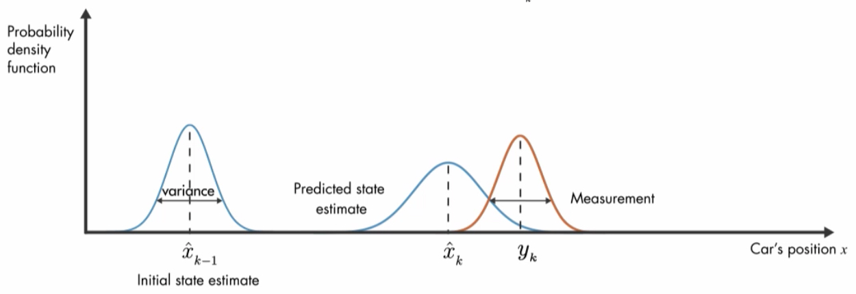
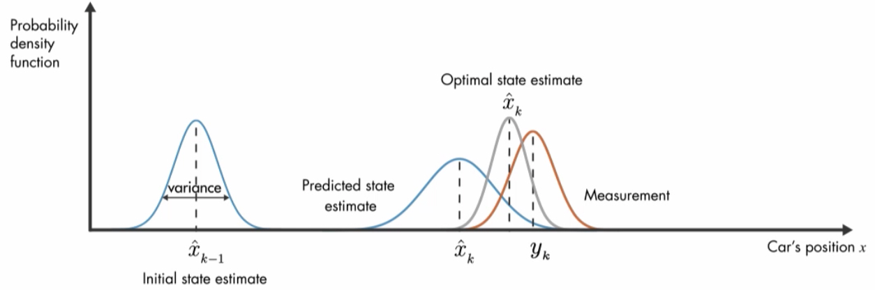
    “Predict-Measure-Update” in 1D

    EECE 5550 Mobile Robotics

    “Predict-Measure-Update” in multivariate

    Transformed prediction from Prior belief

    Giving a new measurement

    Update a Posterior belief

    EECE 5550 Mobile Robotics

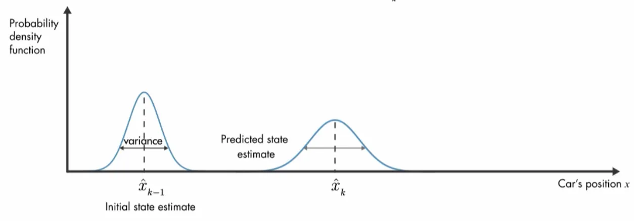
    The recursive Bayes filter: predict, update, repeat

    predict:𝑏𝑒𝑙(xt)=∫p(xt∣ut,xt−1)𝑏𝑒𝑙(xt−1)dxt−1update:𝑏𝑒𝑙(xt)=ηp(zt∣xt)𝑏𝑒𝑙(xt)

    Predict is a blur

    For every place the robot could have been, spread it out by the motion model, and add up. A blur can only widen the belief.

    Update is a reweighting

    Multiply by how well each place explains the reading, then rescale with η. That can only sharpen the belief, or move it.

    p(x∣z)⏟posterior=p(z∣x)⏞likelihoodp(x)⏞priorp(z)

    The recursive Bayes filter: predict, update, repeat

    PREDICTUPDATEUpdated StatePredicted StateInitial stateNew Measurementu: odometryz: LiDAR
    TurtleBot 4
    • odometry predicts at 20 to 62.5 Hz
    • LiDAR updates at about 5 to 10 Hz
    46

    SECTION 5

    The Kalman filter

    The gain as a trust ratio; where Q and R come from

    1D Example

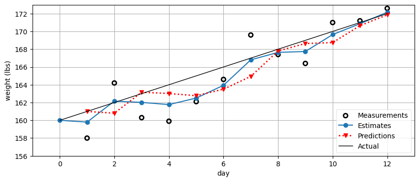
    Measure weight with an imperfect scale

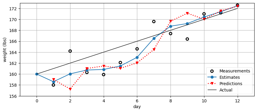
    A person standing on a bathroom scaleMeasurements, estimates, predictions and the true weight over ten days
    Predict:
    prediction = estimate + gain_rate * time_step
    Sensor reading:
    measurement
    Update:
    estimate = prediction + 410(measurement − prediction)
    Giving:
    gain_rate = 1.0 lb/daytime_step = 1.0 day
    What if we have a bad guess?
    48

    EECE 5550 Mobile Robotics

    1D Example

    Measure weight with an imperfect scale

    Previous: we predict a weight gain of 1 lb/day as perfect fitting to the actual gain of truth

    Now: we predict a weight loss of 1 lb/day (-1 lb/day)

    gain_rate: 1 lb/day

    gain_rate: -1 lb/day

    1D Example

    Measure weight with an imperfect scale

    How to fix?
    Compute the gain from existing measurements and estimates!
    A person standing on a bathroom scaleMeasurements, estimates and predictions when the gain is learned from the data
    new gain=old gain+13measurement − predicted weight1 day
    Predict:
    prediction = estimate + gain_rate * time_step
    Sensor reading:
    measurement
    Update:
    estimate = prediction + 410(measurement − prediction)
    Giving:
    gain_rate = 1.0 lb/daytime_step = 1.0 day
    50

    2D Example

    Tracking the constant velocity of an aircraft

    A radar dish tracking an aircraft at two times, t1 and t2, along a straight line
    x˙=v=dxdt
    n12345678910
    zn30171303533075630799310183127831276313793174832175
    xˆn,n30194.230383.6430612.7330818.9331025.731242.331418.831566.331739.431964.1
    x˙ˆn,n39.4238.6542.241.741.5542.4438.934.234.439.67
    xˆn+1,n30391.330576.930823.931027.631233.431454.531613.1531737.2431911.432162.45
    x˙ˆn+1,n39.4238.6542.241.741.5542.4438.934.234.439.67
    ?
    ?
    ?
    ?
    Δt=5s
    xˆ0,0=30,000m
    Predict:
    xˆn,n−1=xˆn−1,n−1+Δtx˙ˆn−1,n−1
    x˙ˆn,n−1=x˙ˆn−1,n−1=40m/s
    State Update Equation
    α=0.2
    β=0.1
    xˆn,n=xˆn,n−1+α(zn−xˆn,n−1)
    x˙ˆn,n=x˙ˆn,n−1+β(zn−xˆn,n−1Δt)
    znMeasurement at time n xˆn,nEstimation of x at time n xˆn+1,nPrediction of x at time n
    xˆ1,0=30,200m
    x˙ˆ1,0=40m/s
    51

    Try it: tune α and β

    α sets how far a residual moves the position estimate; β sets how much it changes the velocity.

    n12345678910
    zn
    xˆn,n
    x˙ˆn,n
    xˆn+1,n
    x˙ˆn+1,n
    52

    g-h filter or α-β filter

    g, h or α, β refer to scaling factors

    xˆn,n=xˆn,n−1+α(zn−xˆn,n−1)x˙ˆn,n=x˙ˆn,n−1+β(zn−xˆn,n−1Δt)
    new gain=old gain+13measurement − predicted weight1 day
    Predict:
    prediction = estimate + gain_rate * time_step
    Sensor reading:
    measurement
    Update:
    estimate = prediction + 410(measurement − prediction)
    Scaling factor g or α
    Scaling factor h or β = 0
    Giving:
    gain_rate = 1.0 lb/daytime_step = 1.0 day
    53

    Kalman filter

    A special case of α-β filter

    KALMAN FILTERMEASUREvalue anduncertaintyUPDATEPREDICTUnit delayn → n − 1OUTPUTSstate estimate,its uncertaintyINITIALIZEinitial state,its uncertaintyestimate
    Rudolf E. Kalman
    Rudolf E. Kalman
    1930-2016
    α-β filter
    State predict
    State update
    xn+1=xn+Δtx˙n
    x˙n+1=x˙n
    xˆn,n=xˆn,n−1+α(zn−xˆn,n−1)x˙ˆn,n=x˙ˆn,n−1+β(zn−xˆn,n−1Δt)
    Kalman filter, one dimension
    State predict
    State update
    xˆn+1,n=xˆn,n+Δtx˙ˆn,n
    x˙ˆn+1,n=x˙ˆn,n
    for constant velocity dynamics
    pn+1,nx=pn,nx+Δt2pn,nv
    pn+1,nv=pn,nv
    for constant velocity dynamics
    xˆn,n=xˆn,n−1+Kn(zn−xˆn,n−1)
    pn,n=(1−Kn)pn,n−1
    Kn=pn,n−1pn,n−1+rn
    54

    Kalman filter

    Prediction Step

    • A general case of prediction matrix Fk:
    • Control matrix Bk and control vector uk
    xk+1=Fkxk+Bkuk
    • Consider both states and covariances:
    • Covariance matrix Σk and process noise matrix Qk
    μk+1=Fkμk+Bkuk,Σk+1=FkΣkFkT+Qk
    PREDICTUPDATEUpdated StatePredicted StateInitial stateNew Measurement
    55

    Kalman filter

    Update Step

    • A general case of measurement model
    • Measurement zk, observation matrix Hk, measurement noise vector δk and measurement noise covariance matrix Rk
    zk=Hkxk+δk,δk∼N(0,Rk)
    • The posterior belief for xk given zk is N(μk,Σk), where:
    μk=μˆk+Kk(zk−Hkμˆk),Σk=(I−KkHk)Σˆk
    • And Kalman Gain as
    Kk=ΣˆkHkT(HkΣˆkHkT+Rk)−1
    PREDICTUPDATEUpdated StatePredicted StateInitial stateNew Measurement
    56

    Kalman filter

    Predict: Given belief xt∼N(μt,Σt) for the current state xt, control ut, and process model:
    xt+1=Atxt+Btut+εt,εt∼N(0,Rt)
    the belief for the next state xt+1 is N(μt+1,Σt+1), where:
    μt+1=Atμt+Btut,Σt+1=AtΣtAtT+Rt
    Update: Given prior belief xt∼N(μˆt,Σˆt) for the current state xt, measurement zt, and measurement model:
    zt=Ctxt+δt,δt∼N(0,Qt)
    the posterior belief for xt given zt is N(μt,Σt), where:
    μt=μˆt+Kt(zt−Ctμˆt),Σt=(I−KtCt)Σˆt
    and
    Kt=ΣˆtCtT(CtΣˆtCtT+Qt)−1
    57

    EECE 5550 Mobile Robotics

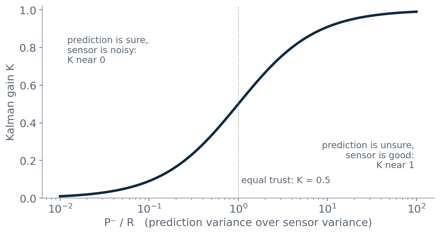
    The gain is a trust ratio

    K near 1

    The prediction is unsure, or the sensor is good. Jump to the measurement.

    K near 0

    The prediction is sure, or the sensor is noisy. Barely move.

    K is not a tuning knob. It is computed every step from P⁻ and r, so it changes as the filter's confidence changes.

    58

    EECE 5550 Mobile Robotics

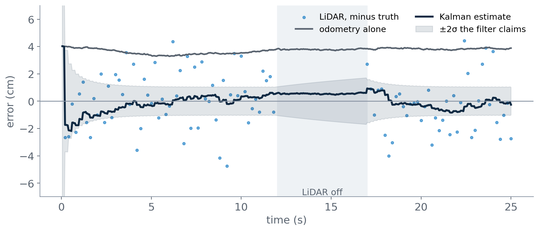
    On the wall: the band collapses on every scan

    Odometry alone keeps its starting error: 3.71 cm RMS. The filter: 0.67 cm. With the LiDAR off, the band widens from 0.51 to 0.85 cm in 5 s, then snaps back.

    59

    A Kalman filter on the distance to a wall

    Your wall_kf.py, running in this page: predict on every odometry step, update on every LiDAR scan.

    LiDAR ON r 2 cm q 1 cm/√m K - σ -
    Python starts when the lecture gets close to this slide.

    Run

    Filter keys from wall_kf

    Python not started yet.
    60

    What wrong noise values do

    Three Kalman filters on one run of wall_kf.py: the same odometry, the same LiDAR scans. Only one noise value differs.

    Mistune by

    Python starts when the lecture gets close to this slide.
    An honest filter keeps the truth inside its own ±2σ band about 95% of the time; far less means a noise value is too small. The values in wall_kf.py come from measurement: r from the LiDAR's spread at a fixed distance, q from the odometry scatter per meter driven.
    Python not started yet.
    61

    EECE 5550 Mobile Robotics

    What to take away

    1

    Every estimate carries a σ.

    A position without an error bar cannot be combined with anything.

    2

    Uncertainty propagates through the math.

    A Σ A-transpose; odometry error grows sideways, as s√s.

    3

    Combining two estimates beats either one.

    Weight by precision, 1/σ², and the result is tighter than the best input.

    4

    The Kalman filter is predict and update, forever.

    Its gain is a trust ratio, computed from Q and R that you measure.

    62